


Next: Update expressions and initial
Up: Second derivative methods
Previous: Rational Function Optimization
Contents
Direct Inversion of Iterative Space (DIIS)
The DIIS method [132] was firstly applied to SCF convergence problems and then
addressed to geometry optimizations [133].
The method is suitable at the vicinity of the stationary point, and it
is based on a linear interpolation/extrapolation of the available structures so as to minimize
the length of an error vector.
The DIIS method minimizing the gradient (GDIIS) has been implemented in section 3.1 in the RFO framework,
therefore it will be briefly described.
We want to obtain a corrected gradient
 as a combination of the previous
  gradient vectors

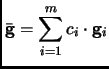 |
(2.80) |
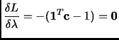
The error function to minimize is
 with the condition

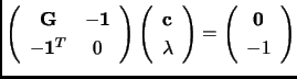
Then, building the corresponding Lagrangian in the matrix form
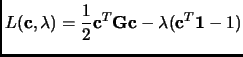 |
(2.81) |
Where
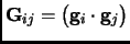 is the matrix containing the scalar products between
the gradients of the last steps.
is the matrix containing the scalar products between
the gradients of the last steps.  is the coefficient vector containing as much components
as iterations. The dimension of matrix
is the coefficient vector containing as much components
as iterations. The dimension of matrix  and vector is equal to the number of iterations.
Derivating 1.81 with respect to
and vector is equal to the number of iterations.
Derivating 1.81 with respect to  and to and imposing the stationary condition
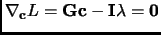 |
(2.82) |
 |
(2.83) |
Joining both derivative conditions in matrix form
 |
(2.84) |
and then
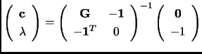 |
(2.85) |
To obtain the coefficients only requires the inversion of a matrix as large as the number of iterations + 1.
From the previous system of equations we can have the improved gradient
and then build up the improved Augmented Hessian
 |
(2.86) |
Next: Update expressions and initial
Up: Second derivative methods
Previous: Rational Function Optimization
Contents
Xavier Prat Resina
2004-09-09