Thermostats and barostats

Using the equations of motion specified above the total energy is a constant of motion. In this case the time averages obtained in this MD simulation are equivalent to ensemble averages in microcanonical ensemble (NVE).

In order to run MD simulation at other non-NVE statistical ensembles we must introduce a thermostat and/or barostat.

Constant Temperature:
The temperature of a particle system is related to the time average of the velocity of the particles

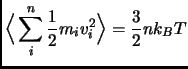$$\Big\langle \sum_i^n \frac{1}{2}m_iv_i^2\Big\rangle = \frac{3}{2}nk_BT$$ (2.105)

The initial velocities can be given from a Maxwell-Boltzmann distribution at the desired temperature. And the most intuitive strategy to keep constant the temperature would be to multiply at every step the velocity of the particles by a scaling factor $\lambda=\sqrt{T_{required}/T_{current}}$.

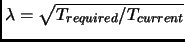Other less rough approaches exist, Andersen introduced the stochastic collisions method[171] and Berendsen and co-workers [172] introduced a coupling parameter $\tau$ to an external bath

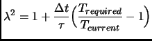$$\lambda^2= 1+ \frac{\Delta t}{\tau}\Bigl(\frac{T_{required}}{T_{current}}-1\Bigr)$$ (2.106)

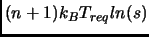
However, the most popular strategy is the extended Lagrangian method that contains additional, artificial coordinates and velocities. It was introduced by Andersen, Nosé[173] and reformulated by Hoover[174]. The reservoir is represented by an additional degree of freedom $s$ with a fictitious mass $Q$ and with potential energy $(n+1)k_BT_{req}ln(s)$. The parameter $Q$ determines the coupling and the energy flow between the reservoir and the real system and therefore the energy oscillations. Some non-ergodicity problems have been reported with Nosé-Hoover method in this case a series of Nosé-Hoover chains are introduced [175,176].

Constant Pressure:
A macroscopic system maintains constant pressure changing its volume. The calculation of the pressure from a particle system is not as direct as the temperature (equation 1.105). The Virial theorem can be used although it can give problems for Periodic Boundary systems.

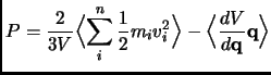$$P=\frac{2}{3V}\Bigl\langle \sum_i^n \frac{1}{2}m_iv_i^2\Bigr\rangle - \Bigl\langle \frac{dV}{d{\bf q}}{\bf q} \Bigr\rangle$$ (2.107)

The amount of volume fluctuation is related to the isothermal compressibility

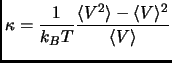$$\kappa = \frac{1}{k_B T}\frac{\langle V^2 \rangle- \langle V \rangle^2}{\langle V \rangle}$$ (2.108)

Many of the methods used for the control of pressure are analogous to those used for the constant temperature. The volume may be changed scaling the positions ${\bf q}_i'=\lambda^{1/3} {\bf q}_i$ of the particles through a coupling parameter $\tau$

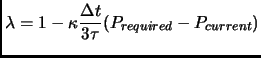$$\lambda=1-\kappa\frac{\Delta t}{3\tau}(P_{required}-P_{current})$$ (2.109)

Otherwise, the Nosé-Hoover scheme can be applied using an external piston as additional degree of freedom [174,177].