However, here we will only cover a very small part of this area that is particularly useful for simulating the localized dynamics of a portion of a protein. This method is very suitable in many enzymatic reactions where the chemical process is expected to take place in a localized region of the enzyme, in this case the expensive Periodic Boundary Conditions may not be necessary and therefore it can be avoided. This is the Stochastic Boundary Molecular Dynamics method (SBMD) [183,184,185,186].
Here we will explain in some detail the SBMD method as it is used in simulations of enzymatic systems [187,188,189] as well as in chapter 4. The SBMD setup has three main characteristics, the partition of the system in three zones, the forces applied to certain zones of the system and the particular equations of motion.
Partitioning the system:
The system is divided in three main regions: dynamics, buffer and reservoir (see figure 1.6).
Dynamics or reaction region: it consists of atoms within a sphere of radius R![]() centered in the active site.
The selection is done by residue, in other words, the entire residue is considered to be in this region if any atom
of the residue falls in the criterion.
This is to avoid disjunct freely floating atoms in the system.
centered in the active site.
The selection is done by residue, in other words, the entire residue is considered to be in this region if any atom
of the residue falls in the criterion.
This is to avoid disjunct freely floating atoms in the system.
Buffer region: which contains the rest of residues surrounding the dynamics region up to a certain distance R![]() (R
(R![]() R
R![]() ).
).
Reservoir region: is the rest of the system, namely, any residue that has all its atoms beyond R![]() distance.
distance.
The atom-labels partitioning the protein are kept fixed all along the simulation while the solvent molecules are
allowed to diffuse between the regions (even between the subpartitions in the buffer region).
Evaluating boundary and stochastic forces:
The atoms that belong to the reservoir region are eliminated2.11.
Therefore, atoms in buffer region must
feel an interaction that reproduces the forces from inexistent reservoir region.
These forces may be divided in average (boundary) forces and stochastic forces.
While reactions in solution the solvent molecules undergo translational diffusion, in proteins the atomic motions have a more localized nature. In this sense the atoms in buffer regions feel a boundary force represented by linear and isotropic restoring forces derived from the atomic mean-square fluctuations. The effective force constant is
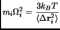 |
(2.111) |
 |
(2.112) |
In addition to the boundary forces it is necessary to mimic the thermal fluctuations, the energy flow between
the buffer and reservoir region. The simplest way to do it is coupling the buffer region to a stochastic heat bath.
This done by ascribing friction coefficients ![]() to the atoms and treating them as interacting Langevin atoms.
The friction coefficient should reproduce the velocity relaxation, and they are computed from the velocity correlation function.
The same friction coefficient is assigned for all the buffer atoms of the protein but considering again the same screening
function as considered in the boundary force. On the contrary, solvent molecules have a constant scaling factor 0.5.
Note that this stochastic heat bath will be used as a thermostat in isothermal ensemble simulations.
to the atoms and treating them as interacting Langevin atoms.
The friction coefficient should reproduce the velocity relaxation, and they are computed from the velocity correlation function.
The same friction coefficient is assigned for all the buffer atoms of the protein but considering again the same screening
function as considered in the boundary force. On the contrary, solvent molecules have a constant scaling factor 0.5.
Note that this stochastic heat bath will be used as a thermostat in isothermal ensemble simulations.
Equations of motion:
Atoms that belong to the dynamics region evolve according to Newton dynamics using a Verlet-type algorithm.
On the other hand, a stochastic dynamics based on the Langevin equation is used for buffer region.
| (2.113) |
The Stochastic Boundary method was designed for reducing the total number of solvent particles included in simulations of localized processes. This reduction must be designed avoiding the spurious edge effects. However, the method does not include the lowest frequency collective motions, this means that the dynamics and buffer regions must be small enough to avoid the necessity of a more sophisticated heat-bath model.
![\includegraphics[width=0.6\textwidth]{Figures/sbmd.eps}](img353.png)