Possible options in the micro-iterative method

Different possible options can be chosen in the general micro-iterative scheme, some of them, as we will see below, may be crucial in order to obtain an accurate convergence as fast as possible.

Frequency of the iterated processes:
Although some authors[108,160] perform a full minimization of the environment at every TS search step, it is not evident that this is the best way to proceed. We could run a full TS search until convergence before minimizing the environment again. As a matter of fact it is still an open question to know which is the most suitable alternating frequency between the two processes.

The core size:
Another important aspect is how big the core zone must be selected in order to reach convergence as fast as possible. When the core is big the coupling between the two search processes is minimized. This would tend to reduce the number of steps required to converge. On the other hand, an optimization of a larger number of atoms requires intrinsically a higher number of steps to converge, in addition a big core region implies a bigger Hessian matrix and, as a consequence, a more expensive initial Hessian calculation (see section 3.4 for a discussion about other problems related to big Hessian matrices).

The interaction between QM and MM zones:
Another option in the micro-iterative method that deserves more discussion is how to handle the interaction between the core and the environment.

The environment zone is usually bigger than the core zone and it needs to be optimized with a cheap minimizer such as conjugate gradient, ABNR or L-BFGS. Although these methods imply low memory requirements their poor efficiency has as a consequence that they need many of steps to reach convergence. Depending on the QM level the environment minimization could demand a high computational effort if a full QM/MM calculation is performed at every step.

Different strategies have been proposed to perform faster QM/MM energy evaluations [249,101,250,84,95,251]. These strategies are based on the idea that an exact SCF evaluation of the QM zone might not be needed at each minimization step in order to calculate the energy of the system. These methods have not only been applied to the location of stationary points [84,95], but also some work had already been done in QM/MM Monte Carlo to explore the environment configurational space avoiding a full SCF evaluation at every step of the simulation[249,101,250,251].

In order to summarize the different approximations adopted to accelerate the QM/MM calculation we have again to keep in mind the general QM/MM electronic embedding scheme already explained in section 1.2.3.1

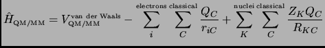
The full Hamiltonian can be expressed as:

$$\hat{H} = \hat{H}_{\mbox{\tiny QM}} + \hat{H}_{\mbox{\tiny MM}} + \hat{H}_{\mbox{\tiny QM/MM}}$$ (4.9)

where $$\hat{H}_{\mbox{\tiny QM}}$$ is the Hamiltonian describing the set of atoms whose interactions are computed using quantum mechanics, and $$\hat{H}_{\mbox{\tiny MM}}$$ is the molecular mechanics Hamiltonian. The crucial aspect is the calculation $$\hat{H}_{\mbox{\tiny QM/MM}}$$ that describes the interaction between the two regions treated at the two different levels

$$\hat{H}_{\mbox{\tiny QM/MM}} = V_{\mbox{\tiny QM/MM}}^{\mbox{\tin... ..._K^{\mbox{\tiny nuclei}} \sum_C^{\mbox{\tiny classical}} \frac{Z_K Q_C}{R_{KC}}$$ (4.10)

where $Q_C$ are the MM charges, $Z_K$ are the effective nuclear charges of quantum atoms, $r_{iC}$ and $R_{KC}$ are the distances from the MM charges to the electrons and quantum nuclei, respectively. The second term of the right-hand of equation 3.10 describes the interaction between the MM charges $Q_C$ and the electrons. The $Q_C$ charges will polarize the wavefunction. So when molecular mechanics atoms are moved all the terms in equation 3.9 have to be recomputed in order to consider the effect of MM atoms on the quantum mechanics zone^4.4. Indeed when the QM level is highly accurate the energy computation becomes not affordable.

ESP:
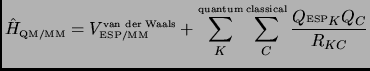
A possible attempt to speed up the full QM/MM calculation is to consider a quantum atom as a classical atom during the MM atoms movement. This can be carried out associating point charges to the quantum atoms, for example, computing the electrostatic potential fitted charges (ESP)[74] from an electron density obtained by means of a full QM/MM calculation. So, in equation 3.10 we can join the second and third term giving the expression shown in equation 3.11

$$\hat{H}_{\mbox{\tiny QM/MM}} = V_{\mbox{\tiny ESP/MM}}^{\mbox{\ti... ...ntum}} \sum_C^{\mbox{\tiny classical}} \frac{Q{\mbox{\tiny ESP}}_K Q_C}{R_{KC}}$$ (4.11)

The ESP charges for the quantum atoms will be constant during the environment minimization and they will be recomputed at the next core step or at the next full QM/MM evaluation. In this case it is evident that the core zone must always include all the quantum atoms.

In this work the ESP charges are taken from a PM3 wavefunction instead of using an ab initio one[84] but this will not include any systematic error in the obtained results.

It is important to note that the ESP/MM strategy will reach a geometry that is not a stationary point on the real QM/MM surface. It is not evident that the interaction between classical charges and ESP charges is equivalent to the second and the third term in equation 3.10. A better approximation is a method which is based on the original QM/MM expression that will be called 1SCF method from here on in this paper.

1SCF:
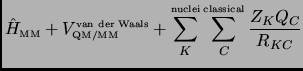
Note that in the QM/MM equation 3.10 the QM/MM interaction Hamiltonian only contributes to the total one-electron core quantum Hamiltonian but not to the two-electron integrals. This means that for a fixed geometry of the quantum atoms if we move the MM atoms the two-electron integrals have not to be recomputed and the one-electron integrals can be easily updated at the new $Q_C$ configuration

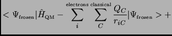
If we save the last converged wave function ( $\Psi_{\mbox{{\tiny frozen}}})$ and perform only one SCF cycle the Fock matrix will not be diagonal but we will obtain a good and cheap approximation to the exact QM/MM energy (see equation 3.12)

$$E_{\mbox{\tiny 1SCF}} = <\Psi_{\mbox{\tiny frozen}} \vert \hat{H}_{\mbox{\tiny QM}} - \su... ...C^{\mbox{\tiny classical}} \frac{Q_C}{r_{iC}}\vert\Psi_{\mbox{\tiny frozen}}> +$$

$$\hat{H}_{\mbox{\tiny MM}} + V_{\mbox{\tiny QM/MM}}^{\mbox{\tiny v... ..._K^{\mbox{\tiny nuclei}} \sum_C^{\mbox{\tiny classical}} \frac{Z_K Q_C}{R_{KC}}$$ (4.12)

Our proposal is to use this method to save computing time during the minimization of the environment in the micro-iterative scheme. The efficiency of this strategy has been evaluated by Evans and Truong [252] in a Monte Carlo sampling of the environment. Keeping the wavefunction frozen will be a good approximation as long as the perturbation of the classical charges $Q_C$ is small. That is, as long as the distribution of charges $Q_C$ during the minimization do not change too much or they are not too close to the QM part to polarize the real $\vert\Psi>$ in a very different manner, the 1SCF method will work well.