Quantum nuclear motion

Assuming that we can solve the electronic Schrödinger equation 1.6 the next step would be to solve the quantum nuclear motion through equation 1.13. In many textbooks we can find an analytical solution to this equation when the PES is a quadratic term. This is the harmonic oscillator and the radial part of the nuclear wavefunctions contains the Hermite polynomial series. This treatment is also valid for the molecular vibrations of the molecule when every normal mode of vibration is assumed to move in a harmonic potential[23].

However, in many cases the harmonic oscillator is far from being adequate and some accurate treatments are needed to solve the nuclear Schrödinger equation and even to contemplate its evolution with time (equation 1.1). See the references [24,25,26,27] for quantum and semi-classical methods used to solve this problem.

In this thesis the nuclei will be considered classical. It means that the nuclear kinetic operator will have the classical form

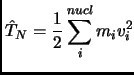$$\hat T_N=\frac{1}{2}\sum_i^{nucl} m_iv_i^2$$ (2.15)

and the nuclear wavefunction $\vert\chi^{nucl}\rangle$ will have no uncertainty in its momenta nor its position. It means that all nuclei can be represented by points of mass $m_i$ and velocity $v_i$ which move, according to equation 1.13, in a potential energy surface. This is usually a good approximation for heavy atoms and high temperatures. When this is not the case the quantum behavior of nuclei should be considered to reproduce purely quantum effects such as tunneling and reflection.