The usual strategy is to consider a non-interacting system whose solution is usually known and then try to solve the real problem by means of perturbation theory or variational theory.
Independent particle model: Hydrogen atom:
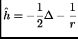
The hydrogen atom was solved analytically by Schrödinger in 1926. Its solution serves as a basis to consider the molecular case[8].
 |
(2.17) |
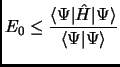
Variational Principle:
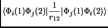
The variational principle states that any wavefunction of the space accomplishes that its expectation value of the energy
is an upper bound to the ground state energy of the system ![]() .
.
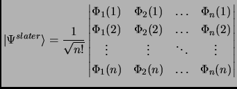
A test function: Slater determinant
An intuitive initial wavefunction would be considering the independent
particle model. That is, a molecule constituted by non-interacting electrons so that every electron will be in an atomic spin-orbital
(from here on ![]() for atoms) or in a molecular spin-orbital (
for atoms) or in a molecular spin-orbital (![]() for molecules).
This choice characterizes the molecular orbital theory.
An alternative to this choice are the Valence Bond Methods where the test function is a combination of configurations
of atomic orbitals. This strategy was named the Heitler-London-Pauling-Slater [8] and during the thirties it was a
good alternative to the molecular orbital theory. However, despite valence bond methods give a chemical vision of the wavefunction
easier to interpret, the numerical convergence is low and quantitative results are expensive.
for molecules).
This choice characterizes the molecular orbital theory.
An alternative to this choice are the Valence Bond Methods where the test function is a combination of configurations
of atomic orbitals. This strategy was named the Heitler-London-Pauling-Slater [8] and during the thirties it was a
good alternative to the molecular orbital theory. However, despite valence bond methods give a chemical vision of the wavefunction
easier to interpret, the numerical convergence is low and quantitative results are expensive.
The operator of non-interacting electrons is a sum of independent one-particle operators and its eigenfunction is the product of the one-particle wavefunctions, this is the so-called Hartree product
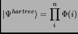 |
(2.19) |
 |
(2.20) |
This can be a good test function, even though it is important to note that we are dealing with only one function of the electronic space (equation 1.16 has infinite solutions), that is, the exact wavefunction for the real system is found in the basis that considers all electrons in all orbitals. It is defined a Slater determinant as a unique configuration. Then the exact solution cannot come from here but when we consider all possible configurations. In section 1.2.1.7 this option is commented as Configuration Interaction.
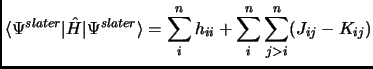
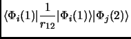
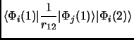
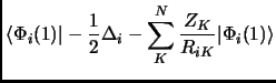
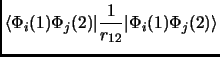
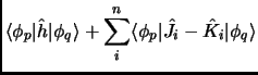
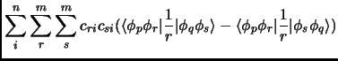
In any case we will see that a Slater determinant is not that bad. So, let us put this Slater determinant in equation 1.18. Considering the orthonormality of the molecular orbitals we obtain the following expressions known as Slater rules[28].
 |
|||
| (2.22) | |||
 |
(2.23) | ||
 |
(2.24) |
Minimization of the energy:
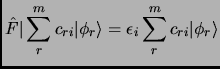
In order to obtain the best molecular orbitals that give the lowest energy we have to minimize
the energy with respect to the orbitals, provided that these orbitals cannot be zero or linear dependent,
that is, constraining the orbitals to be orthogonal and to have a norm of one.
As in many other situations, the optimization of a functional with constraints is carried out by the Lagrange
Multipliers method. Building the Lagrangian ![]() , differentiating with respect to the molecular orbitals and
imposing the stationary conditions (
, differentiating with respect to the molecular orbitals and
imposing the stationary conditions (
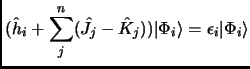
![]() = 0) we could see that the molecular orbitals can be obtained
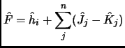
by solving the final Hartree-Fock (HF) equations:
= 0) we could see that the molecular orbitals can be obtained
by solving the final Hartree-Fock (HF) equations:
 |
(2.27) |
Equation 1.29 is a pseudo-eigenvalue equation because the Fock operator cannot be known unless we know the molecular orbitals, and molecular orbitals are obtained by the Fock operator. This dependence (exemplified in equations 1.25 and 1.26) forces that the Hartree-Fock equations must be solved iteratively until self-consistency. This procedure is called Self-Consistent-Field (SCF).
Introduction of a basis: Roothan-Hall equations:
Hartree-Fock equations can only be solved numerically (mapping the orbitals on a set of grid points) for highly
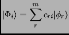
symmetric systems (mostly atoms). In molecular systems we must introduce a known basis set
{
![]() } to span our molecular orbitals as a combination of these
} to span our molecular orbitals as a combination of these ![]() basis functions.
basis functions.
| (2.32) |
 |
(2.33) | ||
 |
(2.34) |
 |
(2.35) |
The method described above is the Restricted Hartree-Fock (RHF), every spin-orbital is a
molecular orbital occupied by two electrons with spin function ![]() and
and ![]() so that the
whole expectation value of spin operator
so that the
whole expectation value of spin operator ![]() is zero.
For open shell systems there are the Restricted Open Shell HF (ROHF) or the more adequate Unrestricted HF method (UHF).
The corresponding Roothan-Hall equations for the UHF case are the Pople-Nesbet equations.
is zero.
For open shell systems there are the Restricted Open Shell HF (ROHF) or the more adequate Unrestricted HF method (UHF).
The corresponding Roothan-Hall equations for the UHF case are the Pople-Nesbet equations.
Few comments about the basis set:
The analytical solution of Hydrogen atom of equation 1.16 has a radial part represented by the Laguerre polynomials
and an angular part represented by the Spherical Harmonics which are basically the associate Legendre Polynomials [8,9].
The basis that we usually introduce in the Roothan-Hall equations will have a radial and an angular part.
The angular is almost never commented because it is always the same (s,p,d,f...). It is the radial part which decides
how far or how close is the electron with respect to the nucleus.
The radial function can be represented by the Slater Type Orbitals (STO).
However, despite of the adequacy of the STO basis, the integrals are not analytical using STO.
Then to avoid expensive numerical integrals it is more common to use Gaussian functions (GTO) which integrals are analytical or
easier to evaluate. In any case some modern methods still employ the STO functions.
Furthermore, the
semiempirical methods used in this thesis are carried out by STO as well. Many textbooks can be found covering the
basis set, the different types, their efficiency and the computational requirements[11].
The SCF process:
We can summarize all the HF process through the Roothan-Hall equations as follows:
It is important to note that the HF method is the best method for a one-configuration wavefunction because we have used the exact electronic Hamiltonian to develop the equations. However there are many improvements to the HF method. Some of them will be outlined very briefly in section 1.2.1.7