General scheme for the strategy

A solution to the storage: limited-memory
We have seen in section 1.3.7.1, where L-BFGS is described, that the limited memory strategy avoids the construction of the Hessian. We store the position and the gradient of a limited number of previous steps and by means of the limited-memory update formulae (equation 1.93 in page ) we could re-build the whole Hessian. Actually we never build the big matrix, but perform the matrix vector product needed to obtain the Newton-Raphson displacement.

Two aspects differentiate the L-BFGS case with ours. i) We want a more accurate control of the curvature of the PES, so it means that we have to deal with the Hessian instead of its inverse. ii)We want an initial Hessian better than a diagonal matrix.

So, if the Hessian we want does not have a trivial inverse it means that we cannot work with original Newton-Raphson equation and its expensive matrix inversion. It turns out that the RFO formulation is a more suitable strategy for this kind of problem^4.8.

The limited-memory-RFO at iteration $k$ would have the known equation already explained in section 3.1

$$\left(\begin{array}{cc} 0 & {\bf g}^T_k \\ {\bf g}_k & {\bf B}_k... ...mbda^{(k)}_\theta {\bf v}^{(k)}_\theta \qquad \forall \quad \theta=1,\ldots,N+1$$ (4.13)

Where in this case the Hessian update is only extended to the last m previous steps.

$${\bf B}_{k+1}={\bf B}_0+\sum_{i=k-m}^k[{\bf j}_i{\bf u}_i^T +{\bf u}_i({\bf j}_i^T -({\bf j}_i^T \Delta {\bf q}_i){\bf u}_i^T )]$$ (4.14)

where ${\bf j}$ and ${\bf u}$ have been explained in page .

The implementation of equations 3.13 and 3.14 would still be problematic because to solve the eigenvalue equation 3.13 we must keep in memory all the matrix. So, we need a diagonalization process able to extract the two lowest eigenpair needed to calculate the displacement without the storage of any big matrix.

A solution to the diagonalization:
iterative diagonalization without storage
A specially suitable solution to this requirement is the family of Lanczos-like diagonalization methods which only require as input a matrix-vector product [254].

In the Normal Mode Analysis the task of diagonalization of a big Hessian is the central computational step [14,255]. There are available on the web free of charge some packages already optimized to solve such big eigenvalue problems. An example of this is the ARPACK and PARPACK. We think that these strategies will give similar results to those we have obtained here.

In the direct multiconfiguration SCF electronic problems big Hamiltonians have to be diagonalized. Iterative diagonalizations have been widely used. Davidson diagonalization is one of the most popular methods. In these kind of problems, only the eigenvalues of the lowest molecular orbitals are needed and the huge Hamiltonian matrix is usually stored in disk rather than in the rapid access memory, so that only matrix-vector product can be calculated.

In the case of geometry optimizations the matrix-vector products can be performed on-the-fly by the update Hessian formula. It is actually the equation 3.14 multiplied by a vector v.

$${\bf B}_{k+1}{\bf v}={\bf B}_0{\bf v}+\sum_{i=k-m}^k[{\bf j}_i{\b... ...bf u}_i({\bf j}_i^T {\bf v}-({\bf j}_i^T \Delta {\bf q}_i){\bf u}_i^T {\bf v})]$$ (4.15)

Note that although we display the expression for the Hessian B$_{k+1}$ actually we have to deal with the diagonalization of the Augmented Hessian of equation 3.13. This is an easy step where the gradient has to be added in the matrix-vector multiplication.

Bofill and co-workers developed an iterative diagonalization method that improves the Davidson method in many aspects [243,256]. It is able to extract not only the lowest or the highest but also the degenerate roots and any eigenpair that fits to a guess given as input. Like all the iterative methods, it is based on the Ritz-Galerkin algorithm. It means that a subspace is constructed where the eigenvalue equation 3.16 is projected and solved. In the Lanczos-like methods this subspace is increased at every iteration. The efficiency of the method will rely on the efficiency of the iterative construction of the subspace basis vectors and the procedure to solve the equation 3.16 in this subspace.

The method developed by Bofill et. al. will not be covered in detail here. Check the references [257,258,243,256] for an accurate description of the equations and the possible alternatives. As a general perspective, the main characteristics of the method are that the vectors to build the iterative subspace are generated first using an approximated or inexact Lagrange-Newton-Raphson (LNR) formula and later, after an orthonormalization procedure, the exact Lagrange-Newton-Raphson equation for the desired root is solved in the iterative subspace.

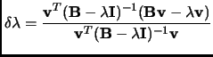
In more detail, we can transform a generic diagonalization problem

$${\bf BV}={\bf V\Lambda}$$ (4.16)

into a minimization process through a Lagrangian function ^4.9:

$$L({\bf v},\lambda)={\bf v}^T{\bf B}{\bf v}-\lambda({\bf v}^{T}{\bf v}-1)$$ (4.17)

Expanding equation 3.17 up to second order and applying the stationary conditions leads to the Lagrange-Newton-Raphson equations. This permits, after some manipulations, to obtain an improvement for the eigenvector ${\bf v}$ and eigenvalue $\lambda$.

$$\delta {\bf v}=-({\bf B}-\lambda{\bf I})^{-1}({\bf Bv}-(\lambda+\delta\lambda){\bf v})$$ (4.18)

$$\delta\lambda=\frac{{\bf v}^T({\bf B}-\lambda{\bf I})^{-1}({\bf Bv}-\lambda{\bf v})}{{\bf v}^T({\bf B} - \lambda{\bf I})^{-1}{\bf v}}$$ (4.19)

A critical point is also the inversion of the full matrix in the denominator of equation 3.19 that can be approximated by a diagonal(Davidson) or by a square+vector (figure 3.1 in page ).

This iterative diagonalization task involves a sort of internal optimization process to obtain every new vector of the subspace. Such internal optimization of the subspace basis vector is carried out by Newton-Raphson method or by a Rational Function Optimization. Note that in equation 3.18 ${\bf B}-\lambda{\bf I}$ would be the Hessian and ${\bf Bv}-(\lambda+\delta\lambda){\bf v}$ the gradient. This is important because if the iterative diagonalization process takes many steps to converge the subspace will increase its dimension and the internal Hessian diagonalizations could become problematic.

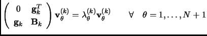
As a resume the procedure of diagonalization of a matrix B can be outlined as follows:

1. Start with a normalized guess eigenvector v. Compute the corresponding eigenvalue $\lambda={\bf v^TBv}$
2. Using the inexact LNR equations 3.18 and 3.19 compute the improvements to v and $\lambda$. (they are inexact because involve the inversion of the big matrix that must be approximated by its diagonal or the square+vector form)
3. Orthonormalize the new improved vector with the rest of the already constructed subspace, through a Gramm-Schmidt procedure [259] for example.
4. Project the LNR equations to the subspace and solve it by a Newton-Raphson or RFO procedure.
5. The solution of this internal optimization will be the improvement $\delta {\bf v}$ to the initial eigenvector v.
6. If this improvement is bigger than a convergence criteria, return to point 1. If not, the whole process is ended with the eigenpair (v,$\lambda$) as a result.

If the convergence is reached after $k$ iterations the number of matrix-vector products ${\bf Bv}$ will be $k+1$. The algorithm only needs to store three vectors in the high speed memory at every iteration.