 |
(2.120) |
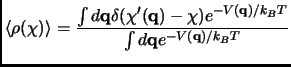
In a more practical way, the PMF can be used to know how the free energy changes as a function of a coordinate of the system. It can be a geometrical coordinate or a more general energetic (solvent) coordinate. Unlike the mutations used frequently in free energy perturbation calculations which are often along non-physical pathways, the PMF is usually calculated for a physical achievable process. In particular it is useful for predicting the rates in chemical solution and for elucidating the reaction mechanism of condensed phase reaction such as enzymatic processes.
The PMF ![]() along some coordinate
along some coordinate ![]() is defined from the average distribution function
is defined from the average distribution function
![]()
![$\displaystyle w(\chi) = w(\chi^*) - k_BT\ln\Bigl[\frac{\langle \rho (\chi)\rangle}{\langle \rho (\chi^*)\rangle} \Bigr]$](img396.png) |
(2.121) |
Where
![]() is the Dirac delta function for the coordinate
is the Dirac delta function for the coordinate ![]() . We are assuming
that the chosen coordinate
. We are assuming
that the chosen coordinate ![]() is a geometrical coordinate
is a geometrical coordinate
![]() , but
, but ![]() can have any other functionality.
For processes with an activation barrier higher than k
can have any other functionality.
For processes with an activation barrier higher than k![]() T the distribution function
T the distribution function
![]() cannot be computed by a straight molecular dynamics simulation.
Such computation would not converge due to low sampling in higher-energy configurations.
Special sampling techniques (non-Boltzmann sampling) have been developed to obtain a PMF along a coordinate
cannot be computed by a straight molecular dynamics simulation.
Such computation would not converge due to low sampling in higher-energy configurations.
Special sampling techniques (non-Boltzmann sampling) have been developed to obtain a PMF along a coordinate ![]() .
Although PMF of enzymatic reactions can be calculated using free energy perturbation [112,188,195],
the method used in this thesis and explained here is the Umbrella Sampling technique [196,197].
.
Although PMF of enzymatic reactions can be calculated using free energy perturbation [112,188,195],
the method used in this thesis and explained here is the Umbrella Sampling technique [196,197].
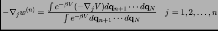
Umbrella Sampling:
In this method, the microscopic system is simulated in the presence of an artificial biasing window potential ![]() that is added to the potential energy
that is added to the potential energy
![]() .
.
| (2.123) |
Unless the entire range of ![]() coordinate is spanned in a single simulation,
multiple simulations (windows) are performed with different biasing umbrella potentials
coordinate is spanned in a single simulation,
multiple simulations (windows) are performed with different biasing umbrella potentials
![]() that center the sampling
in different overlapping regions or windows of
that center the sampling
in different overlapping regions or windows of ![]() .
.
A reasonable choice to produce the biased ensembles, though not the unique2.12,
is to use for every window ![]() an harmonic function of the form
an harmonic function of the form
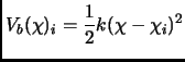 |
(2.124) |
At every window ![]() the distribution function is efficiently converged
the distribution function is efficiently converged
![]() through the expression of the distribution function in equation 1.122
substituting
through the expression of the distribution function in equation 1.122
substituting
![]() for
for
![]() .
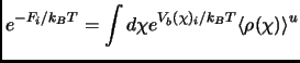
The superindices
.
The superindices ![]() and
and ![]() indicate biased and unbiased respectively.
The distribution functions from the various windows need to be unbiased
indicate biased and unbiased respectively.
The distribution functions from the various windows need to be unbiased
![]() (the non-Boltzmann factor is removed)
and then recombined together to obtain the final estimate PMF
(the non-Boltzmann factor is removed)
and then recombined together to obtain the final estimate PMF ![]() . Otherwise, obtaining the unbiased PMF for the
. Otherwise, obtaining the unbiased PMF for the ![]() window
window
![$\displaystyle w(\chi)_i^u = w(\chi^*) - k_BT\ln\Bigl[\frac{\langle \rho (\chi)\rangle_i^b}{\langle \rho (\chi^*)\rangle} \Bigr] - V_b(\chi)_i + F_i$](img412.png) |
(2.125) |
| (2.126) |
A more sophisticated strategy is the Weighted Histogram Analysis Method (WHAM) [198] that makes usage of all the information in the umbrella sampling, and does not discard the overlapping regions. In addition, WHAM does not require a significant amount of overlap and it can be easily extended to multi-dimensional PMF [199,200].
In particular the WHAM technique computes the total unbiased distribution function
![]() as a weighted sum of the unbiased distribution functions
as a weighted sum of the unbiased distribution functions
![]() .
This weighting function can be expressed in terms of the known biased distribution functions
.
This weighting function can be expressed in terms of the known biased distribution functions
![]()
See reference [201] for a comparative study between the different techniques to unbias and recombine the data extracted from Umbrella Sampling.
![$\displaystyle \langle \rho (\chi) \rangle^u = \sum_{i=1}^N n_i \langle \rho (\c...
..._i^b \times \Bigl [ \sum_{j=1}^N n_j e^{-(V_b(\chi)_i - F_i)/k_BT} \Bigr ]^{-1}$](img418.png)