Results and discussion

Location of the minima:
Although nowadays several cheap and efficient minimization algorithms exist, we present here the comparative results between our algorithm and two others that are widely used. To this aim we carried out geometry minimizations with our algorithm (RFO-m-BFGS) and two quasi-Newton-Raphson algorithms. These two quasi-Newton-Raphson algorithms use the BFGS and the L-BFGS update Hessian matrix formula. These two algorithms, which were also coupled to the Roar-cp module, are labeled qNR-BFGS and qNR-L-BFGS. The results corresponding to the minimizations with the L-BFGS update formula were obtained using information from the five previous iterations. After several tests this number of iterations was proven to be the best compromise between the efficiency of the method and memory requirements.

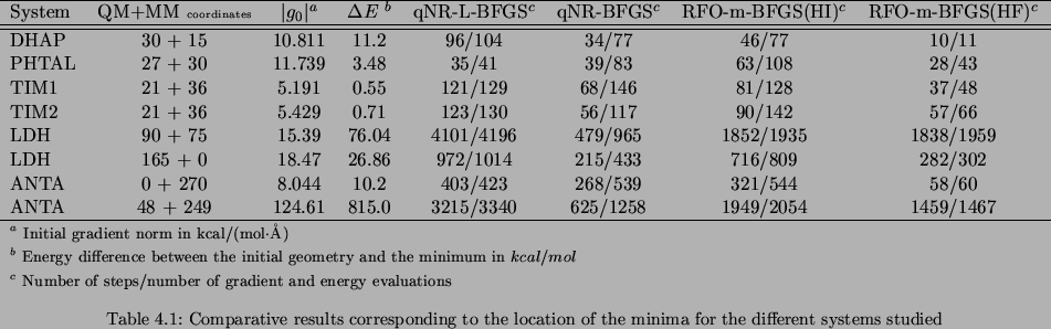
The comparative results for the search for the minima are presented in table 3.1. We are able to choose the minimization algorithm between qNR-BFGS, qNR-L-BFGS and RFO-m-BFGS. As we said the unity matrix is taken as the initial guess Hessian matrix for qNR-BFGS and qNR-L-BFGS. For the sake of comparison we used two different initial guess Hessian matrices for RFO-m-BFGS. So, RFO-m-BFGS(HI) stands for the RFO-m-BFGS algorithm with the unity matrix as an initial guess, whereas the initial Hessian matrix for the RFO-m-BFGS(HF) algorithm was calculated numerically according to equation 1.70 in page building up a matrix of the form shown in figure 3.1 (except for the ANTA system when the whole system is treated classically).

In each system the minimum reached by all of the algorithms is always the same. So we just specify the energy difference between the starting point and the minimum reached. A final numerical Hessian calculation was done in order to characterize the stationary point. The convergence criterion on the root mean square (RMS) of the gradient is 10$^{-3}$ kcal/(moli$\cdot$Å), except for ANTA, which is 10$^{-4}$ kcal/(mol$\cdot$Å). We also present the number of steps and the number of energy and gradient evaluations (the energy and gradient calculations required to build up the numerical initial guess Hessian matrix are not counted). This information will give us the efficiency of every step. Note that the energy and the gradient are calculated only once each step unless the displacement vector needs to be corrected. This is why the number of steps is always smaller than the number of energy and gradient calculations, as seen in table 3.1.

No global conclusions about the compared efficiency between the different algorithms can be drawn. We can just note a general tendency because the behavior of an optimization depends not only on the algorithm but also on the intrinsic characteristics of the system (size, starting point, fixed atoms and convergence criteria). Nevertheless it can be seen that qNR-L-BFGS tends to need more steps than the other algorithms. This is due to the fact that it only works with the information of the last five preceding steps.

Comparing the results for the columns corresponding to the RFO-m-BFGS(HI) and RFO-m-BFGS(HF) algorithms, there is an evident conclusion. When an initial Hessian matrix is calculated numerically the number of steps and the energy and gradient evaluations required decrease compared to when the starting Hessian matrix is a unity matrix. It can be seen that RFO-m-BFGS(HF) behaves reasonably well in comparison with qNR-BFGS. In addition, bearing in mind that the number of energy and gradient evaluations compared to the number of steps indicates the efficiency of the step, it is shown that the efficiency of an RFO-m-BFGS(HF) step is greater than that of a qNR-BFGS step because the ratio between those two numbers for qNR-BFGS is always more than 2, whereas the ratio for the RFO-m-BFGS(HF) algorithm is close to 1.

Figure 3.4: Gradient RMS (kcal mol$^{-1}$ $\cdot$ Å$^{-1}$) for the QM/MM ANTA system as a function of the number of steps of minimization with four algorithms

We also studied how the RMS of the gradient behaves during the minimization process. Although we present here only the QM/MM ANTA system as an illustrative example (figure 3.4) the comparative results are similar in all the systems studied. It can be seen that the RFO-m-BFGS(HF) algorithm reaches a low-gradient region faster, and it is in this quasi-converged region where it spends most of the steps. This is true even for the cases for which qNR-BFGS needs fewer steps to reach the minimum. The reason why RFO-m-BFGS(HF) reaches a low-gradient zone faster is obviously due to the information that provides the initially calculated Hessian matrix and probably the higher RFO efficiency. The reason why once in a quasi-converged RMS gradient region, RFO-m-BFGS(HF) can sometimes require many steps could be due to a a recognized behavior of RFO and consequently it does not give the correct shift [245].

Location of transition states:
We report the test of the RFO-Powell algorithm with the same reactive systems as for the minima in table 3.2. We recall that for a transition-state search the BFGS formula cannot be used because, in the TS case, the M matrix involved in equation 3.5 is not positive-definite.

Table 3.2: Results corresponding to the location of transition states for the different systems studied

System	QM+MM coordinates	$\vert g_0\vert$$^a$	$\Delta E$ $^b$	RFO-Powell(HF)$^c$
DHAP	30+15	6.86	22.82	56/59
PHTAL	27+30	1.18	4.03	39/54
TIM	21+36	11.17	3.70	65/88
LDH	165+0	6.78	4.19	614/636
LDH	36+129	3.24	0.87	316/392
ANTA	0+270	8.04	7.78	291/315
ANTA	48+249	2.10	1.25	421/598
$^a$ Initial gradient norm in $kcal/(mol\cdot\AA)$
$^b$ Energy difference between the initial geometry and the minimum in $kcal/mol$
$^c$ Number of steps/number of gradient and energy evaluations

The initial structure for the transition-state search is usually the most energetic point in a few points scan along the approximated reaction path. During the search we have to ensure that the algorithm is following the correct direction. This direction will be given by the eigenvector with the negative eigenvalue of the current Hessian matrix (Augmented Hessian in our case). In order to follow during the search the same direction, we choose the eigenvector with the maximum overlap with the followed eigenvector of the previous step.

Once the transition state is reached we have characterized the structure found by a numerical calculation of the Hessian matrix.

Overall, the RFO-Powell algorithm performs well in locating transition states. The ratio between the number of steps and the number of gradient and energy evaluations is still close to 1 as previously found during the minimization process. Our implementation allows the location of transition-state structures, even if they are quite far away from the starting structures as depicted in table 3.2 for the DHAP system (i.e, $\Delta E=22.82$ $kcal/mol$). Therefore, we can deduce from the previous results that the RFO-Powell algorithm is a solid algorithm to locate transition-state structures of systems from small to medium size, involving different ratios of QM and MM atoms, described in Cartesian coordinates, including link atoms and representing several types of chemical reactions.